Studying CNTK (6): ResNet

To unleash the power of image recognition you still need the ResNet architecture, first proposed by Microsoft Research Asia. This network structure can achieve recognition rates above 90%—for example, ResNet CIFAR-10 needs as many as 21 convolutional layers, with batch renormalization and normalization redone at every step.

In August 2016 Google open-sourced Inception-ResNet-v2, built on TensorFlow, with even stronger recognition that can accurately classify Alaska Malamutes (left) from Siberian Huskies. There are also V3 and V4, with deeper architectures. Notably, Inception-v4 has no residual connections but matches V2's performance.

But these are things personal computers struggle to run. CNTK also has various ResNet implementations; the default ResNet20_CIFAR10.cntk runs 160 iterations. The compute load is huge and very slow, but recognition accuracy is extremely high—still well worth trying.

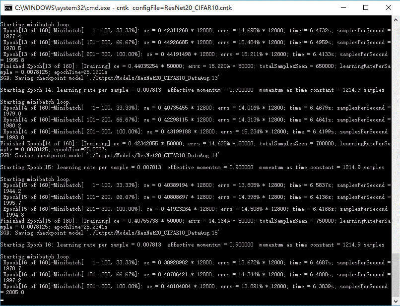
By the 16th iteration accuracy already exceeds 86.1%. Each iteration takes about 25s, so only a few minutes total. Its rate of accuracy improvement is even faster than a simple convolutional network. Around 28 iterations it reaches about 89–90% recognition; truly breaking 90% is roughly at 36 iterations—about 15 minutes to hit 90%, entirely acceptable. But according to the docs, training to the end still bottoms out around an 8.2% error rate, while humans are estimated at about 6%—this architecture alone still cannot surpass humans. Stacking to n=18, however, reaches 6.2–6.5%. A quick test showed one epoch of that network takes about 153 seconds; 160 iterations take roughly 6.8 hours to reach 6.2–6.5%.

 

According to research that has been done, more layers is not always better for ResNet.

At 1202 layers, performance is actually worse than at 110 layers.

 

A comparison:

ResNet20_CIFAR10, numLayers = 3, learningRatesPerMB = 1.0*80:0.1*40:0.01

ResNet18_CIFAR10, numLayers = 18, learningRatesPerMB = 0.1*1:1.0*80:0.1*40:0.01

Apart from these, there is no difference.

So it is enough to analyze the source file ResNet20_CIFAR10.cntk.

# ConvNet applied on CIFAR-10 dataset, with data augmentation (translation and flipping).

command = TrainConvNet:Eval

precision = "float"; traceLevel = 1 ; deviceId = "auto"

rootDir = "../.." ; configDir = "./" ; dataDir = "$rootDir$/DataSets/CIFAR-10" ;
outputDir = "./Output" ;

modelPath = "$outputDir$/Models/ResNet20_CIFAR10_DataAug"
#stderr = "$outputDir$/ResNet20_CIFAR10_DataAug_bs_out"

TrainConvNet = {
 action = "train"

 BrainScriptNetworkBuilder = {
 include "$configDir$/Macros.bs" 

 imageShape = 32:32:3 # images all resized to 32
 labelDim = 10 # only ten classification categories

 featScale = 1/256
 Normalize{f} = x => f .* x

 cMap = 16:32:64
 bnTimeConst = 4096
 numLayers = 3
 
 model = Sequential (
 Normalize {featScale} :

 ConvBNReLULayer {cMap[0], (3:3), (1:1), bnTimeConst} :
 ResNetBasicStack {numLayers, cMap[0], bnTimeConst} :

 ResNetBasicInc {cMap[1], (2:2), bnTimeConst} :
 ResNetBasicStack {numLayers-1, cMap[1], bnTimeConst} :
 
 ResNetBasicInc {cMap[2], (2:2), bnTimeConst} :
 ResNetBasicStack {numLayers-1, cMap[2], bnTimeConst} :
 
 # avg pooling
 AveragePoolingLayer {(8: 8), stride = 1} :
 LinearLayer {labelDim}
 )

 # inputs
 features = Input {imageShape}
 labels   = Input {labelDim}

 # apply model to features
 z = model (features)

 # connect to system
 ce = CrossEntropyWithSoftmax (labels, z)
 errs = ClassificationError (labels, z)
 top5Errs = ClassificationError (labels, z, topN=5)  # only used in Eval action

 featureNodes = (features)
 labelNodes = (labels)
 criterionNodes  = (ce)
 evaluationNodes = (errs)  # top5Errs only used in Eval
 outputNodes = (z)
 }

 SGD = {
 epochSize = 0
 minibatchSize = 128

 # Note that learning rates are 10x more than in the paper due to a different
 # momentum update rule in CNTK: v{t + 1} = lr*(1 - momentum)*g{t + 1} + momentum*v{t}

 # The learning rates here are 10x those in the paper; things differ slightly. Automatic learning-rate variation uses a momentum approach—Nesterov Momentum, based on convex optimization theory, has better convergence.
 learningRatesPerMB = 1.0*80:0.1*40:0.01
 momentumPerMB = 0.9

 # number of iterations
 maxEpochs = 160

 # L2 regularization weight; for details see: https://msdn.microsoft.com/zh-cn/dn904675.aspx
 L2RegWeight = 0.0001

 numMBsToShowResult = 100
 }

 reader = {
 verbosity = 0 ; randomize = true
 deserializers = ({
 type = "ImageDeserializer" ; module = "ImageReader"
 file = "$dataDir$/train_map.txt"
 input = {
 features = { transforms = (
 { type = "Crop" ; cropType = "random" ; cropRatio = 0.8 ; jitterType = "uniRatio" } :
 { type = "Scale" ; width = 32 ; height = 32 ; channels = 3 ; interpolations = "linear" } :
 { type = "Mean" ; meanFile = "$dataDir$/CIFAR-10_mean.xml" } :
 { type = "Transpose" }
 )}
 labels = { labelDim = 10 }
 }
 })
 }
}

# Eval action
Eval = {
 action = "eval"
 evalNodeNames = errs:top5Errs  # also test top-5 error rate
 # Set minibatch size for testing.
 minibatchSize = 128

 reader = {
 verbosity = 0 ; randomize = false
 deserializers = ({
 type = "ImageDeserializer" ; module = "ImageReader"
 file = "$dataDir$/test_map.txt"
 input = {
 features = { transforms = (
 { type = "Scale" ; width = 32 ; height = 32 ; channels = 3 ; interpolations = "linear" } :
 { type = "Mean"; meanFile = "$dataDir$/CIFAR-10_mean.xml" } :
 { type = "Transpose" }
 )}
 labels = { labelDim = 10 }
 }
 })
 }
}